Variational Bayesian methods

Variational Bayesian methods, also called 'ensemble learning', are a family of techniques for approximating intractable integrals arising in Bayesian inference and machine learning. They are typically used in complex statistical models consisting of observed variables (usually termed "data") as well as unknown parameters and latent variables, with various sorts of relationships among the three types of random variables, as might be described by a graphical model. As is typical in Bayesian inference, the parameters and latent variables are grouped together as "unobserved variables". Variational Bayesian methods can provide an analytical approximation to the posterior probability of the unobserved variables, and also to derive a lower bound for the marginal likelihood (sometimes called the "evidence") of several models (i.e. the marginal probability of the data given the model, with marginalization performed over unobserved variables), with a view to performing model selection. It is an alternative to Monte Carlo sampling methods for taking a fully Bayesian approach to statistical inference over complex distributions that are difficult to directly evaluate or sample from.

Variational Bayes can be seen as an extension of the EM (expectation-maximization) algorithm from maximum a posteriori estimation (MAP estimation) of the single most probable value of each parameter to fully Bayesian estimation which computes(an approximation to) the entire posterior distribution of the parameters and latent variables.

1 Mathematical derivation
2 In practice
3 A simple example
4 A more complex example
5 Exponential-family distributions
6 See also
7 Notes
8 References
9 External links

Mathematical derivation

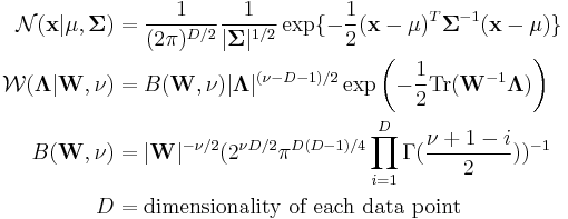
In variational inference, the posterior distribution over a set of unobserved variables $\mathbf{Z} = \{Z_1 \dots Z_n\}$ given some data $\mathbf{X}$ is approximated by a variational distribution, $Q(\mathbf{Z})$ :

$P(\mathbf{Z}|\mathbf{X}) \approx Q(\mathbf{Z}).$

The distribution $Q(\mathbf{Z})$ is restricted to belong to a family of distributions of simpler form than $P(\mathbf{Z}|\mathbf{X})$ , selected with the intention of making $Q(\mathbf{Z})$ similar to the true posterior, $P(\mathbf{Z}|\mathbf{X})$ . The lack of similarity is measured in terms of a dissimilarity function $d(Q; P)$ and hence inference is performed by selecting the distribution $Q(\mathbf{Z})$ that minimizes $d(Q; P)$ . One choice of dissimilarity function that makes this minimization tractable is the Kullback–Leibler divergence (KL divergence) of P from Q, defined as

$D_{\mathrm{KL}}(Q || P) = \sum_\mathbf{Z} Q(\mathbf{Z}) \log \frac{Q(\mathbf{Z})}{P(\mathbf{Z}|\mathbf{X})}.$

This can be written as

$D_{\mathrm{KL}}(Q || P) = \sum_\mathbf{Z} Q(\mathbf{Z}) \log \frac{Q(\mathbf{Z})}{P(\mathbf{Z},\mathbf{X})} %2B \log P(\mathbf{X}),$

$\begin{align} \log P(\mathbf{X}) & = D_{\mathrm{KL}}(Q||P) - \sum_\mathbf{Z} Q(\mathbf{Z}) \log \frac{Q(\mathbf{Z})}{P(\mathbf{Z},\mathbf{X})} \\ & = D_{\mathrm{KL}}(Q||P) %2B \mathcal{L}(Q). \end{align}$

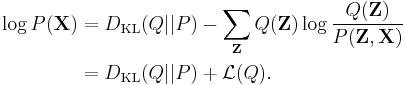
As the so-called log evidence $\log P(\mathbf{X})$ is fixed with respect to $Q$ , maximising the final term $\mathcal{L}(Q)$ minimizes the KL divergence of $P$ from $Q$ . By appropriate choice of $Q$ , $\mathcal{L}(Q)$ becomes tractable to compute and to maximize. Hence we have both an analytical approximation $Q$ for the posterior $P(\mathbf{Z}|\mathbf{X})$ , and a lower bound $\mathcal{L}(Q)$ for the evidence $\log P(\mathbf{X})$ . The lower bound $\mathcal{L}(Q)$ is known as the (negative) variational free energy because it can also be expressed as an "energy" $\operatorname{E}_{Q}[\log P(\mathbf{Z},\mathbf{X})]$ plus the entropy of $Q$ .

In practice

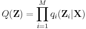
The variational distribution $Q(\mathbf{Z})$ is usually assumed to factorize over some partition of the latent variables, i.e. for some partition of the latent variables $\mathbf{Z}$ into $\mathbf{Z}_1 \dots \mathbf{Z}_M$ ,

$Q(\mathbf{Z}) = \prod_{i=1}^M q_i(\mathbf{Z}_i|\mathbf{X})$

It can be shown using the calculus of variations (hence the name "variational Bayes") that the "best" distribution $q_j^{*}$ for each of the factors $q_j$ (in terms of the distribution minimizing the KL divergence, as described above) can be expressed as:

$q_j^{*}(\mathbf{Z}_j|\mathbf{X}) = \frac{e^{\operatorname{E}_{i \neq j} [\ln p(\mathbf{Z}, \mathbf{X})]}}{\int e^{\operatorname{E}_{i \neq j} [\ln p(\mathbf{Z}, \mathbf{X})]}\, d\mathbf{Z}_j}$

where $\operatorname{E}_{i \neq j} [\ln p(\mathbf{Z}, \mathbf{X})]$ is the expectation of the joint probability of the data and latent variables, taken over all variables not in the partition.

In practice, we usually work in terms of logarithms, i.e.:

$\ln q_j^{*}(\mathbf{Z}_j|\mathbf{X}) = \operatorname{E}_{i \neq j} [\ln p(\mathbf{Z}, \mathbf{X})] %2B \text{constant}$

The constant in the above expression is related to the normalizing constant (the denominator in the expression above for $q_j^{*}$ ) and is usually reinstated by inspection, as the rest of the expression can usually be recognized as being a known type of distribution (e.g. Gaussian, gamma, etc.).

Using the properties of expectations, the expression $\operatorname{E}_{i \neq j} [\ln p(\mathbf{Z}, \mathbf{X})]$ can usually be simplified into a function of the fixed hyperparameters of the prior distributions over the latent variables and of expectations (and sometimes higher moments such as the variance) of latent variables not in the current partition (i.e. latent variables not included in $\mathbf{Z}_j$ ). This creates circular dependencies between the parameters of the distributions over variables in one partition and the expectations of variables in the other partitions. This naturally suggests an iterative algorithm, much like EM (the expectation-maximization algorithm), in which the expectations (and possibly higher moments) of the latent variables are initialized in some fashion (perhaps randomly), and then the parameters of each distribution are computed in turn using the current values of the expectations, after which the expectation of the newly computed distribution is set appropriately according to the computed parameters. An algorithm of this sort is guaranteed to converge.^[1] Furthermore, if the distributions in question are part of the exponential family, which is usually the case, convergence will be to a global maximum, since the exponential family is convex.^[2]

In other words, for each of the partitions of variables, by simplifying the expression for the distribution over the partition's variables and examining the distribution's functional dependency on the variables in question, the family of the distribution can usually be determined (which in turn determines the value of the constant). The formula for the distribution's parameters will be expressed in terms of the prior distributions' hyperparameters (which are known constants), but also in terms of expectations of functions of variables in other partitions. Usually these expectations can be simplified into functions of expectations of the variables themselves (i.e. the means); sometimes expectations of squared variables (which can be related to the variance of the variables), or expectations of higher powers (i.e. higher moments) also appear. In most cases, the other variables' distributions will be from known families, and the formulas for the relevant expectations can be looked up. However, those formulas depend on those distributions' parameters, which depend in turn on the expectations about other variables. The result is that the formulas for the parameters of each variable's distributions can be expressed as a series of equations with mutual, nonlinear dependencies among the variables. Usually, it is not possible to solve this system of equations directly. However, as described above, the dependencies suggest a simple iterative algorithm, which in most cases is guaranteed to converge. An example will make this process clearer.

A simple example

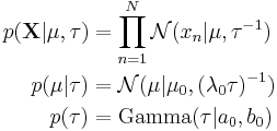
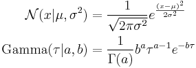
Imagine a simple Bayesian model consisting of a single node with a Gaussian distribution, with unknown mean and precision (or equivalently, an unknown variance, since the precision is the reciprocal of the variance).^[3]

We place conjugate prior distributions on the unknown mean and variance, i.e. the mean also follows a Gaussian distribution while the precision follows a gamma distribution. In other words:

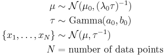
$\begin{align} \mu & \sim \mathcal{N}(\mu_0, (\lambda_0 \tau)^{-1}) \\ \tau & \sim \operatorname{Gamma}(a_0, b_0) \\ \{x_1, \dots, x_N\} & \sim \mathcal{N}(\mu, \tau^{-1}) \\ N &= \text{number of data points} \end{align}$

We are given $N$ data points 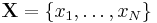$\mathbf{X} = \{x_1, \dots, x_N\}$ and our goal is to infer the posterior distribution $q(\mu, \tau)=p(\mu,\tau|x_1, \ldots, x_N)$ of the parameters $\mu$ and $\tau$ .

The hyperparameters $\mu_0$ , $\lambda_0$ , $a_0$ and $b_0$ are fixed, given values. They can be set to small positive numbers to give broad prior distributions indicating ignorance about the prior distributions of $\mu$ and $\tau$ .

The joint probability of all variables can be rewritten as

$p(\mathbf{X},\mu,\tau) = p(\mathbf{X}|\mu,\tau) p(\mu|\tau) p(\tau)$

where the individual factors are

$\begin{align} p(\mathbf{X}|\mu,\tau) & = \prod_{n=1}^N \mathcal{N}(x_n|\mu,\tau^{-1}) \\ p(\mu|\tau) & = \mathcal{N}(\mu|\mu_0, (\lambda_0 \tau)^{-1}) \\ p(\tau) & = \operatorname{Gamma}(\tau|a_0, b_0) \end{align}$

where

$\begin{align} \mathcal{N}(x|\mu,\sigma^2) & = \frac{1}{\sqrt{2\pi\sigma^2}} e^\frac{(x-\mu)^2}{2\sigma^2} \\ \operatorname{Gamma}(\tau|a,b) & = \frac{1}{\Gamma(a)} b^a \tau^{a-1} e^{-b \tau} \end{align}$

Assume that 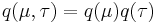$q(\mu,\tau) = q(\mu)q(\tau)$ , i.e. that the posterior distribution factorizes into independent factors for $\mu$ and $\tau$ . This type of assumption underlies the variational Bayesian method. The true posterior distribution does not in fact factor this way (in fact, in this simple case, it is known to be a Gaussian-gamma distribution), and hence the result we obtain will be an approximation.

Then

$\begin{align} \ln q_\mu^*(\mu) &= \operatorname{E}_{\tau}[\ln p(\mathbf{X}|\mu,\tau) %2B \ln p(\mu|\tau)] %2B \text{constant} \\ &= - \frac{\operatorname{E}[\tau]}{2} \{ \lambda_0(\mu-\mu_0)^2 %2B \sum_{n=1}^N (x_n-\mu)^2 \} %2B \text{constant} \end{align}$

Note that the term $\operatorname{E}_{\tau}[\ln p(\tau)]$ will be a function solely of $a_0$ and $b_0$ and hence is constant with respect to $\mu$ ; thus it has been absorbed into the constant term at the end. By expanding the squares inside of the braces, separating out and grouping the terms involving $\mu$ and $\mu^2$ and completing the square over $\mu$ , we see that $q_\mu^*(\mu)$ is a Gaussian distribution 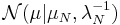$\mathcal{N}(\mu|\mu_N,\lambda_N^{-1})$ where we have defined:

$\begin{align} \mu_N &= \frac{\lambda_0 \mu_0 %2B N \bar{x}}{\lambda_0 %2B N} \\ \lambda_N &= (\lambda_0 %2B N) \operatorname{E}[\tau] \end{align}$

Similarly,

$\begin{align} \ln q_\tau^*(\tau) &= \operatorname{E}_{\mu}[\ln p(\mathbf{X}|\mu,\tau) %2B \ln p(\mu|\tau)] %2B \ln p(\tau) %2B \text{constant} \\ &= (a_0 - 1) \ln \tau - b_0 \tau %2B \frac{N}{2} \ln \tau - \frac{\tau}{2} \operatorname{E}_\mu [\sum_{n=1}^N (x_n-\mu)^2 %2B \lambda_0(\mu - \mu_0)^2] %2B \text{constant} \end{align}$

Exponentiating both sides, we can see that $q_\tau^*(\tau)$ is a gamma distribution $\operatorname{Gamma}(\tau|a_N, b_N)$ where we have defined

$\begin{align} a_N &= a_0 %2B \frac{N%2B1}{2} \\ b_N &= b_0 %2B \frac{1}{2} \operatorname{E}_\mu \left[\sum_{n=1}^N (x_n-\mu)^2 %2B \lambda_0(\mu - \mu_0)^2\right] \end{align}$

In each case, the parameters for the distribution over one of the variables depend on expectations taken with respect to the other variable. The formulas for the expectations of moments of the Gaussian and gamma distributions are well-known, but depend on the parameters. Hence the formulas for each distribution's parameters depend on the other distribution's parameters. This naturally suggests an EM-like algorithm where we first initialize the parameters to some values (perhaps the values of the hyperparameters of the corresponding prior distributions) and iterate, computing new values for each set of parameters using the current values of the other parameters. This is guaranteed to converge to a local maximum, and since both posterior distributions are in the exponential family, this local maximum will be a global maximum.

Note also that the posterior distributions have the same form as the corresponding prior distributions. We did not assume this; the only assumption we made was that the distributions factorize, and the form of the distributions followed naturally. It turns out (see below) that the fact that the posterior distributions have the same form as the prior distributions is not a coincidence, but a general result whenever the prior distributions are members of the exponential family, which is the case for most of the standard distributions.

A more complex example

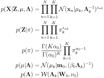
Imagine a Bayesian Gaussian mixture model described as follows:

$\begin{align} \mathbf{\pi} & \sim \operatorname{SymDir}(K, \alpha_0) \\ \mathbf{\Lambda}_{i=1 \dots K} & \sim \mathcal{W}(\mathbf{W}_0, \nu_0) \\ \mathbf{\mu}_{i=1 \dots K} & \sim \mathcal{N}(\mathbf{\mu}_0, (\beta_0 \mathbf{\Lambda}_i)^{-1}) \\ \mathbf{z}[i = 1 \dots N] & \sim \operatorname{Mult}(1, \mathbf{\pi}) \\ \mathbf{x}_{i=1 \dots N} & \sim \mathcal{N}(\mathbf{\mu}_{z_i}, {\mathbf{\Lambda}_{z_i}}^{-1}) \\ K &= \text{number of mixing components} \\ N &= \text{number of data points} \end{align}$

Note:

SymDir() is the symmetric Dirichlet distribution of dimension $K$ , with the hyperparameter for each component set to $\alpha_0$ . The Dirichlet distribution is the conjugate prior of the categorical distribution or multinomial distribution.
$\mathcal{W}()$ is the Wishart distribution, which is the conjugate prior of the precision matrix (inverse covariance matrix) for a multivariate Gaussian distribution.
Mult() is a multinomial distribution over a single observation. The state space is a "one-of-K" representation, i.e. a $K$ -dimensional vector in which one of the elements is 1 (specifying the identity of the observation) and all other elements are 0.
$\mathcal{N}()$ is the Gaussian distribution, in this case specifically the multivariate Gaussian distribution.

The interpretation of the above variables is as follows:

$\mathbf{X} = \{\mathbf{x}_1, \dots, \mathbf{x}_N\}$ is the set of $N$ data points, each of which is a $K$ -dimensional vector distributed according to a multivariate Gaussian distribution.
$\mathbf{Z} = \{\mathbf{z}_1, \dots, \mathbf{z}_N\}$ is a set of latent variables, one per data point, specifying which mixture component the corresponding data point belongs to, using a "one-of-K" vector representation with components $z_{nk}$ for $k = 1 \dots K$ , as described above.
$\mathbf{\pi}$ is the mixing proportions for the $K$ mixture components.
$\mathbf{\mu}_{i=1 \dots K}$ and $\mathbf{\Lambda}_{i=1 \dots K}$ specify the parameters (mean and precision) associated with each mixture component.

The joint probability of all variables can be rewritten as

$p(\mathbf{X},\mathbf{Z},\mathbf{\pi},\mathbf{\mu},\mathbf{\Lambda}) = p(\mathbf{X}|\mathbf{Z},\mathbf{\mu},\mathbf{\Lambda}) p(\mathbf{Z}|\mathbf{\pi}) p(\mathbf{\pi}) p(\mathbf{\mu}|\mathbf{\Lambda}) p(\mathbf{\Lambda})$

where the individual factors are

$\begin{align} p(\mathbf{X}|\mathbf{Z},\mathbf{\mu},\mathbf{\Lambda}) & = \prod_{n=1}^N \prod_{k=1}^K \mathcal{N}(\mathbf{x}_n|\mathbf{\mu}_k,\mathbf{\Lambda}_k^{-1})^{z_{nk}} \\ p(\mathbf{Z}|\mathbf{\pi}) & = \prod_{n=1}^N \prod_{k=1}^K \pi_k^{z_{nk}} \\ p(\mathbf{\pi}) & = \frac{\Gamma(K\alpha_0)}{\Gamma(\alpha_0)^K} \prod_{k=1}^K \pi_k^{\alpha_0-1} \\ p(\mathbf{\mu}|\mathbf{\Lambda}) & = \mathcal{N}(\mathbf{\mu}_k|\mathbf{m}_0,(\beta_0 \mathbf{\Lambda}_k)^{-1}) \\ p(\mathbf{\Lambda}) & = \mathcal{W}(\mathbf{\Lambda}_k|\mathbf{W}_0, \nu_0) \end{align}$

where

$\begin{align} \mathcal{N}(\mathbf{x}|\mathbf{\mu},\mathbf{\Sigma}) & = \frac{1}{(2\pi)^{D/2}} \frac{1}{|\mathbf{\Sigma}|^{1/2}} \exp \{-\frac{1}{2}(\mathbf{x}-\mathbf{\mu})^T \mathbf{\Sigma}^{-1}(\mathbf{x}-\mathbf{\mu}) \} \\ \mathcal{W}(\mathbf{\Lambda}|\mathbf{W},\nu) & = B(\mathbf{W},\nu) |\mathbf{\Lambda}|^{(\nu-D-1)/2} \exp \left(-\frac{1}{2} \operatorname{Tr}(\mathbf{W}^{-1}\mathbf{\Lambda}) \right) \\ B(\mathbf{W},\nu) & = |\mathbf{W}|^{-\nu/2} (2^{\nu D/2} \pi^{D(D-1)/4} \prod_{i=1}^{D} \Gamma(\frac{\nu %2B 1 - i}{2}))^{-1} \\ D & = \text{dimensionality of each data point} \end{align}$

Assume that $q(\mathbf{Z},\mathbf{\pi},\mathbf{\mu},\mathbf{\Lambda}) = q(\mathbf{Z})q(\mathbf{\pi},\mathbf{\mu},\mathbf{\Lambda})$ .

Then

$\begin{align} \ln q^*(\mathbf{Z}) &= \operatorname{E}_{\mathbf{\pi},\mathbf{\mu},\mathbf{\Lambda}}[\ln p(\mathbf{X},\mathbf{Z},\mathbf{\pi},\mathbf{\mu},\mathbf{\Lambda})] %2B \text{constant} \\ &= \operatorname{E}_{\mathbf{\pi}}[\ln p(\mathbf{Z}|\mathbf{\pi})] %2B \operatorname{E}_{\mathbf{\mu},\mathbf{\Lambda}}[\ln p(\mathbf{X}|\mathbf{Z},\mathbf{\mu},\mathbf{\Lambda})] %2B \text{constant} \\ &= \sum_{n=1}^N \sum_{k=1}^K z_{nk} \ln \rho_{nk} %2B \text{constant} \end{align}$

where we have defined

$\ln \rho_{nk} = \operatorname{E}[\ln \pi_k] %2B \frac{1}{2} \operatorname{E}[\ln |\mathbf{\Lambda}_k|] - \frac{D}{2} \ln(2\pi) - \frac{1}{2} \operatorname{E}_{\mathbf{\mu}_k,\mathbf{\Lambda}_k} [(\mathbf{x}_n - \mathbf{\mu}_k)^T \mathbf{\Lambda}_k (\mathbf{x}_n - \mathbf{\mu}_k)]$

Exponentiating both sides of the formula for $\ln q^*(\mathbf{Z})$ yields

$q^*(\mathbf{Z}) \propto \prod_{n=1}^N \prod_{k=1}^K \rho_{nk}^{z_{nk}}$

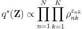
Requiring that this be normalized ends up requiring that the $\rho_{nk}$ sum to 1 over all values of $k$ , yielding

$q^*(\mathbf{Z}) = \prod_{n=1}^N \prod_{k=1}^K r_{nk}^{z_{nk}}$

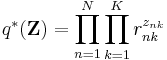
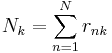
where

$r_{nk} = \frac{\rho_{nk}}{\sum_{j=1}^K \rho_{nj}}$

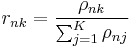
In other words, $q^*(\mathbf{Z})$ is a product of single-observation multinomial distributions, and factors over each individual $\mathbf{z}_n$ , which is distributed as a single-observation multinomial distribution with parameters $r_{nk}$ for $k = 1 \dots K$ .

Furthermore, we note that

$\operatorname{E}[z_{nk}] = r_{nk} \,$

which is a standard result for categorical distributions.

Now, considering the factor $q(\mathbf{\pi},\mathbf{\mu},\mathbf{\Lambda})$ , note that it automatically factors into 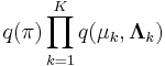$q(\mathbf{\pi}) \prod_{k=1}^K q(\mathbf{\mu}_k,\mathbf{\Lambda}_k)$ due to the structure of the graphical model defining our Gaussian mixture model, which is specified above.

Then,

$\begin{align} \ln q^*(\mathbf{\pi}) &= \ln p(\mathbf{\pi}) %2B \operatorname{E}_{\mathbf{Z}}[\ln p(\mathbf{Z}|\mathbf{\pi})] %2B \text{constant} \\ &= (\alpha_0 - 1) \sum_{k=1}^K \ln \pi_k %2B \sum_{n=1}^N \sum_{k=1}^K r_{nk} \ln \pi_k %2B \text{constant} \end{align}$

Taking the exponential of both sides, we recognize $q^*(\mathbf{\pi})$ as a Dirichlet distribution

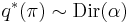
$q^*(\mathbf{\pi}) \sim \operatorname{Dir}(\mathbf{\alpha}) \,$

where

$\alpha_k = \alpha_0 %2B N_k \,$

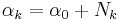
where

$N_k = \sum_{n=1}^N r_{nk} \,$

Finally

$\ln q^*(\mathbf{\mu}_k,\mathbf{\Lambda}_k) = \ln p(\mathbf{\mu}_k,\mathbf{\Lambda}_k) %2B \sum_{n=1}^N \operatorname{E}[z_{nk}] \ln \mathcal{N}(\mathbf{x}_n|\mathbf{\mu}_k,\mathbf{\Lambda}_k^{-1}) %2B \text{constant}$

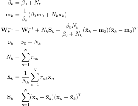
Grouping and reading off terms involving $\mathbf{\mu}_k$ and $\mathbf{\Lambda}_k$ , the result is a Gaussian-Wishart distribution given by

$q^*(\mathbf{\mu}_k,\mathbf{\Lambda}_k) = \mathcal{N}(\mathbf{\mu}_k|\mathbf{m}_k,(\beta_k \mathbf{\Lambda}_k)^{-1}) \mathcal{W}(\mathbf{\Lambda}_k|\mathbf{W}_k,\nu_k)$

given the definitions

$\begin{align} \beta_k &= \beta_0 %2B N_k \\ \mathbf{m}_k &= \frac{1}{\beta_k} (\beta_0 \mathbf{m}_0 %2B N_k {\bar{\mathbf{x}}}_k) \\ \mathbf{W}_k^{-1} &= \mathbf{W}_0^{-1} %2B N_k \mathbf{S}_k %2B \frac{\beta_0 N_k}{\beta_0 %2B N_k} ({\bar{\mathbf{x}}}_k - \mathbf{m}_0)({\bar{\mathbf{x}}}_k - \mathbf{m}_0)^T \\ \nu_k &= \nu_0 %2B N_k \\ N_k &= \sum_{n=1}^N r_{nk} \\ {\bar{\mathbf{x}}}_k &= \frac{1}{N_k} \sum_{n=1}^N r_{nk} \mathbf{x}_n \\ \mathbf{S}_k &= \sum_{n=1}^N (\mathbf{x}_n - {\bar{\mathbf{x}}}_k) (\mathbf{x}_n - {\bar{\mathbf{x}}}_k)^T \end{align}$

Finally, notice that these functions require the values of $r_{nk}$ , which make use of $\rho_{nk}$ , which is defined in turn based on $\operatorname{E}[\ln \pi_k]$ , $\operatorname{E}[\ln |\mathbf{\Lambda}_k|]$ , and $\operatorname{E}_{\mathbf{\mu}_k,\mathbf{\Lambda}_k} [(\mathbf{x}_n - \mathbf{\mu}_k)^T \mathbf{\Lambda}_k (\mathbf{x}_n - \mathbf{\mu}_k)]$ . Now that we have determined the distributions over which these expectations are taken, we can derive formulas for them:

$\begin{array}{rcccl} \operatorname{E}_{\mathbf{\mu}_k,\mathbf{\Lambda}_k} [(\mathbf{x}_n - \mathbf{\mu}_k)^T \mathbf{\Lambda}_k (\mathbf{x}_n - \mathbf{\mu}_k)] &&&=& D\beta_k^{-1} %2B \nu_k (\mathbf{x}_n - \mathbf{m}_k)^T \mathbf{W}_k (\mathbf{x}_n - \mathbf{m}_k) \\ \ln {\tilde{\Lambda}}_k &\equiv& \operatorname{E}[\ln |\mathbf{\Lambda}_k|] &=& \sum_{i=1}^D \psi \left(\frac{\nu_k %2B 1 - i}{2}\right) %2B D \ln 2 %2B \ln |\mathbf{\Lambda}_k| \\ \ln {\tilde{\pi}}_k &\equiv& \operatorname{E}\left[\ln |\pi_k|\right] &=& \psi(\alpha_k) - \psi\left(\sum{i=1}^K \alpha_i\right) \end{array}$

These results lead to

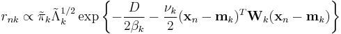
$r_{nk} \propto {\tilde{\pi}}_k {\tilde{\Lambda}}_k^{1/2} \exp \left\{ - \frac{D}{2 \beta_k} - \frac{\nu_k}{2} (\mathbf{x}_n - \mathbf{m}_k)^T \mathbf{W}_k (\mathbf{x}_n - \mathbf{m}_k) \right\}$

These can be converted from proportional to absolute values by normalizing over $k$ so that the corresponding values sum to 1.

Note that:

The update equations for the parameters $\beta_k$ , $\mathbf{m}_k$ , $\mathbf{W}_k$ and $\nu_k$ of the variables $\mathbf{\mu}_k$ and $\mathbf{\Lambda}_k$ depend on the statistics $N_k$ , ${\bar{\mathbf{x}}}_k$ , and $\mathbf{S}_k$ , and these statistics in turn depend on $r_{nk}$ .
The update equations for the parameters $\alpha_{1 \dots K}$ of the variable $\mathbf{\pi}$ depend on the statistic $N_k$ , which depends in turn on $r_{nk}$ .
The update equation for $r_{nk}$ has a direct circular dependence on $\beta_k$ , $\mathbf{m}_k$ , $\mathbf{W}_k$ and $\nu_k$ as well as an indirect circular dependence on $\mathbf{W}_k$ , $\nu_k$ and $\alpha_{1 \dots K}$ through ${\tilde{\pi}}_k$ and ${\tilde{\Lambda}}_k$ .

This suggests an iterative procedure that alternates between two steps:

An E-step that computes the value of $r_{nk}$ using the current values of all the other parameters.
An M-step that uses the new value of $r_{nk}$ to compute new values of all the other parameters.

Note that these steps correspond closely with the standard EM algorithm to derive a maximum likelihood or maximum a posteriori (MAP) solution for the parameters of a Gaussian mixture model. The responsibilities $r_{nk}$ in the E step correspond closely to the posterior probabilities of the latent variables given the data, i.e. $p(\mathbf{Z}|\mathbf{X})$ ; the computation of the statistics $N_k$ , ${\bar{\mathbf{x}}}_k$ , and $\mathbf{S}_k$ corresponds closely to the computation of corresponding "soft-count" statistics over the data; and the use of those statistics to compute new values of the parameters corresponds closely to the use of soft counts to compute new parameter values in normal EM over a Gaussian mixture model.

Exponential-family distributions

Note that in the previous example, once the distribution over unobserved variables was assumed to factorize into distributions over the "parameters" and distributions over the "latent data", the derived "best" distribution for each variable was in the same family as the corresponding prior distribution over the variable. This is a general result that holds true for all prior distributions derived from the exponential family.

Notes

^ Boyd, Stephen P.; Vandenberghe, Lieven (2004) (pdf). Convex Optimization. Cambridge University Press. ISBN 9780521833783. http://www.stanford.edu/~boyd/cvxbook/bv_cvxbook.pdf. Retrieved October 15, 2011.
^ Christopher Bishop, Pattern Recognition and Machine Learning, 2006
^ Based on Chapter 10 of Pattern Recognition and Machine Learning by Christopher M. Bishop

References

Bishop, Christopher M. (2006). Pattern Recognition and Machine Learning. Springer. ISBN 0-387-31073-8.

External links

Variational-Bayes Repository A repository of papers, software, and links related to the use of variational methods for approximate Bayesian learning
The on-line textbook: Information Theory, Inference, and Learning Algorithms, by David J.C. MacKay provides an introduction to variational methods (p. 422).
Variational Algorithms for Approximate Bayesian Inference, by M. J. Beal includes comparisons of EM to Variational Bayesian EM and derivations of several models including Variational Bayesian HMMs.

Variational Bayesian methods

Contents

Mathematical derivation

In practice

A simple example

A more complex example

Exponential-family distributions

See also

Notes

References

External links